March 27, 2024

PlonK Deconstructed: Math Toolkit for KZG

Benjamin Bencik

plonk elliptic-curves

In this part, we will cover basics of the mathematical background needed for KZG polynomial commitment sheme. Fully understanding it requires a bit of preliminaries. We will try to be brief, so let's get this out of the way.

Elliptic Curves

An elliptic curve is defined as $f(x,y): y^2 = x^3 + ax + b$ with parameters $a, b$. When plotted over the real numbers, it might look like one of the images below, depending on the choice of parameters.

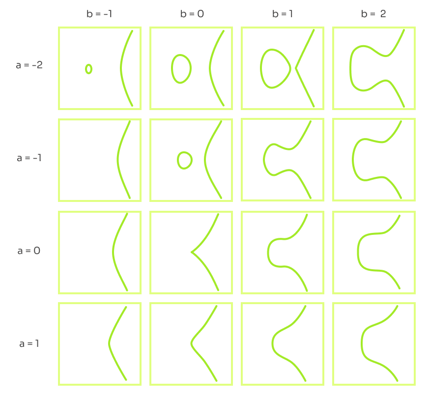
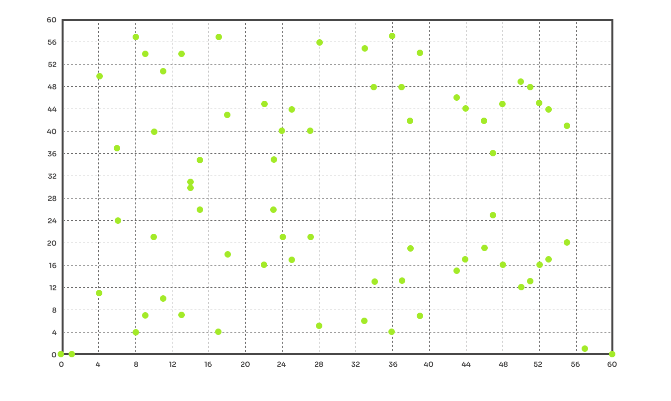
Points of the elliptic curve are in the usual form $(x \text{ coordinate}, y \text{ coordinate})$. We will be interested in elliptic curves over a finite field $\mathbb{F}_p$ where $p$ is a prime number. Essentially this means that the coordinates $(x, y)$ are both from the set $[0, 1, 2, \ldots, p-1]$. Moreover, for any two elements of $\mathbb{F}_p$ we can perform addition and multiplication under modulo $p$. Finite fields have other special features but we will not get into it. We use elliptic curves over finite fields partly because for computers it is easier to perform arithmetic operations on integers than on real numbers. To make it a bit less abstract, below is an elliptic curve with parameters $a = -1, b = 0$ over the finite field $\mathbb{F}_{61}$.

Any two points of an elliptic curve can be added and also subtracted in specific way. For this construction, there hold certain nice properties. For example, adding or subtracting any two points on the curve results in another point on the same elliptic curve. These properties could be generalized by mathematical object group. A standard group needs to be defined on some set $\mathbb{G}$ and a group operation $\circ$. So, we can say that the set of points of an elliptic curve over a finite field with operation addition form a group. Groups are not anything super fancy and we encounter them daily. For example, the set of whole numbers $\mathbb{Z}$ with operation $+$ also forms a group. The nice thing is that groups are well-studied mathematical object. By showing that elliptic curves form a group we can use any statement (theorem) about groups and apply it to elliptic curves.

A group needs to have a single neutral element $e$ and each element needs to have assigned a single inverse element. Performing the group operation $\circ$ on any element $x \in \mathbb{G}$ with a neutral element $e$ simply results in $x$. For inverse, it holds that the operation of an element with an inverse element results in a neutral element: $\forall x \in \mathbb{G}: x \circ x^{-1} = e$. The subtraction of elements $a, b$ can be written as $a \circ b^{-1}$. This might sound complicated but it is not. In the example on whole numbers $\mathbb{Z}$ with $+$ the neutral element $e$ is 0 and inverse elements are negative numbers. Taking any number from $\mathbb{Z}$ and adding to its inverse naturally results in zero, which indeed is the neutral element for $\mathbb{Z}$ with $+$. For the group formed by an elliptic curve points the the neutral element $e$ is the point at infinity $(0,0)$ and the inverse to $(x,y)$ is $(x,-y)$.

It is also possible to perform exponentiation which is just a repeated application of the group operation $\circ$. So $\forall x \in \mathbb{G}$ the exponentiation $x^k$ is $x \circ x \circ ... \circ x$ applied $k$ times. But remember that group, by definition, has only a single operation $\circ$, and exponentiation is just notation convenience. The are two common notations for the operation of the group formed by points of an elliptic curve. Some use additive notation where $\circ$ is $+$ and some multiplicative notation where $\circ$ is $\times$. We will stick with multiplicative but it is just a matter of preference. Besides that we will need a group generator $G$. That is an element of the group that generates the whole group by exponentiation. In other words, if $G$ is a generator then the whole group could be expressed as $\{G^1, G^2, G^3, \ldots, G^{p-1}\}$.

Discrete Logarithm Problem

Why all of the hassle with elliptic curves? It is all because of the Discrete Logarithm Problem (DLP) which is considered to be hard on elliptic curves. Given $x, y \in \mathbb{G}$ such that $x^k = y $ it is hard to find $k$. Of course, the hardness depends on the size of $\mathbb{G}$. The bigger the group the harder it is to solve the problem. It is similar to passwords, the longer your password is the harder it is for someone to guess it.

While calculating $y$ from $x, k$ is straightforward, we do not know any efficient algorithm to calculate $k$ from $x, y$. This is a standard assumption in cryptography and many modern protocols are based on the hardness of DLP. To make things clear, DLP is not impossible to solve but hard to solve efficiently in reasonable amount of time. If we base the hardness of the protocol on the hardness of DLP, then our protocol is hard to break as long as no one can efficiently compute DLP on elliptic curves. Note that the DLP is specifically hard to compute on group formed by an elliptic curve, but for $\mathbb{Z}$ with $+$ it is simple.

Elliptic curve operations

In the KZG we will want to encode polynomial evaluations as elements of the elliptic curve group. For now, take that as a fact, we will describe the construction of these polynomials in the following posts. You will shortly see that if we take an evaluation $f(a)$ we can encode them as a group element $G^{f(a)}$ where $G$ is the generator of some group $\mathbb{G}$. Elliptic curves will turn out to be very useful because thanks to the DLP the evaluation $f(a)$ can encrypted as $G^{f(a)}$. This is not so special on its own. However, what is special is that one can get secret values $(a, b, \ldots)$ encoded as elliptic curve points $(G^a, G^b, \ldots)$ and still perform some operation with them without discovering the secret values $(a, b, \ldots)$. In the context of zero-knowledge protocol, the prover might send polynomial evaluations encoded as elliptic curve points, and the verifier can perform arithmetic operations without discovering the actual values.

Let's sum up which operations we can use. Given values $(a, b, \ldots)$ encoded as elliptic curve points $(G^a, G^b, \ldots)$ one can perform these operations "in the exponent":

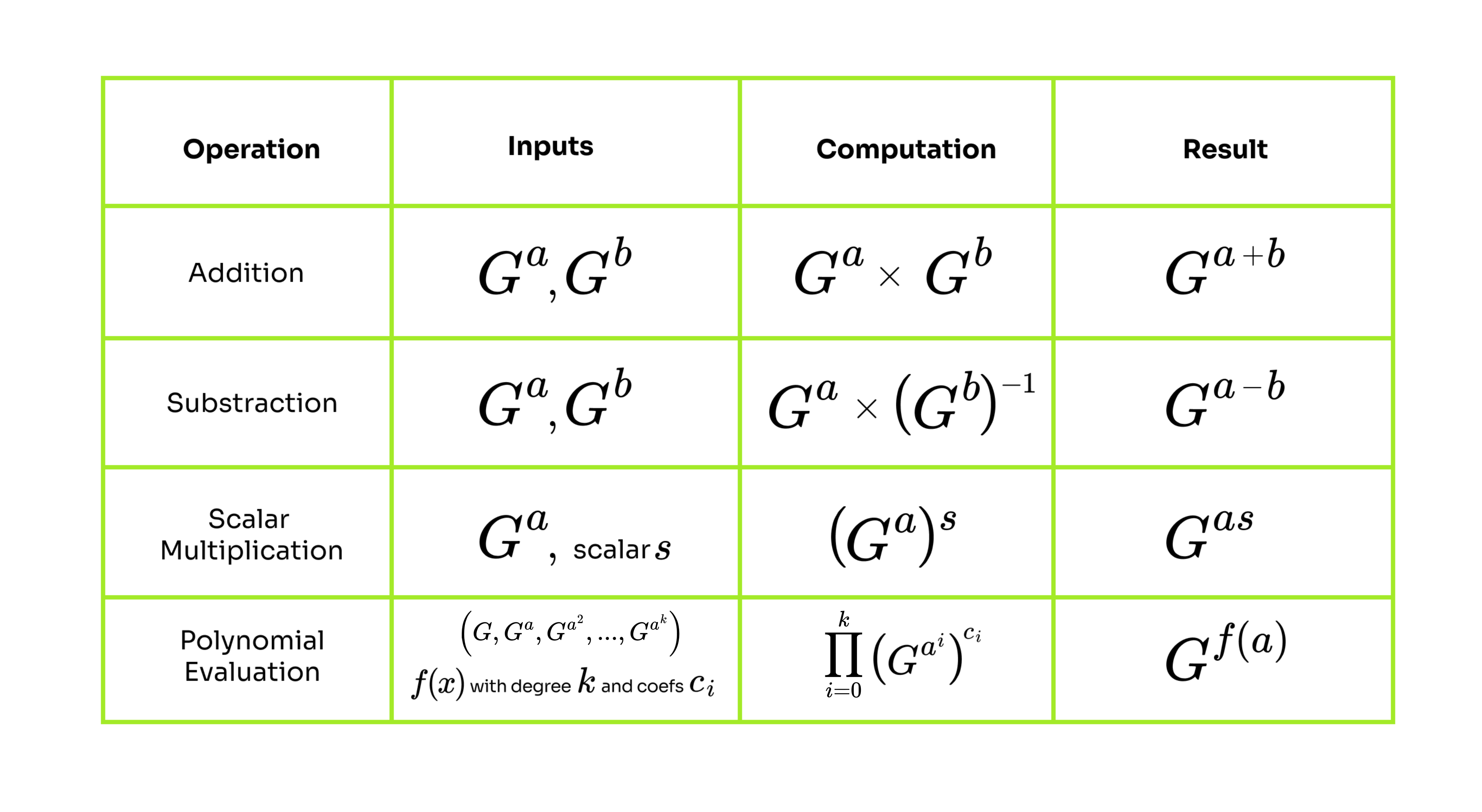
The first row just described the standard group operation. In the second row, we first take the inverse of the operand and perform the group operation. Scalar multiplication is just a generalization of exponentiation. For the polynomial evaluation, we need to realize that any polynomial $f(x)$ of degree $k$ can be written in form $f(x) = c_0 + c_1 x + c_2 x^2 + ... + c_k x^k$. That means evaluation of $f(x)$ at some point $a$ can be written as:

This can be split into terms as:

Curve Pairings

Fully understanding curve pairings takes quite a bit of advanced algebra, so we will simplify a lot. Essentially curve pairing $e$ takes two points $p \in \mathbb{G}_1, q \in \mathbb{G}_2$ and maps them to some other target group. That is all.

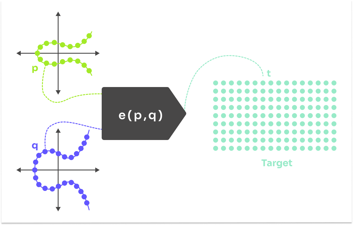
We will use the pairing as black-box, and it will be enough to know that they the following properties:

If you look at the table of operation, notice that we cannot compute $G^{a \times b}$ given $G^a, G^b$. This operation is needed in the verification of KZG. And pairings solve exactly this problem. By taking $G_1^a, G_2^b$ we can calculate $G_t^{a \times b}$ in the target group.

Pairing-friendly curves do not occur that often out in the wild. That is why well-known curves are usually used. One example is BLS12-381. If you want to learn more check out amazing post BLS12-381 For The Rest Of Us.

Comparing polynomials

The last piece of the puzzle is being able to compare two polynomials. We will do this by comparing them at a single point. At first sight, this seems like the most naive approach, however, for a large enough domain, it works overwhelmingly well.

Why is it sufficient to compare polynomials at a single point? (optional section)

We will demonstrate a case on polynomials with single variable $x$. If the polynomials are identical then for sure $\forall x: f(x) = g(x)$ and this check always accepts. However, this check might also accept polynomials that differ but have intersection at the randomly picked point. To calculate the probability of failure we would like to know the upper bound of intersections of two different polynomials.

Take two arbitrary polynomials $p(x) = a_0 + a_1x + a_2x^2 ... a_nx^n = 0$ and $q(x) = b_0 + b_1x + b_2x^2 ... b_m x^m = 0$ with degree $n, m$ that are no bigger than some degree bound $d \leq \mathbb{N}$. Without the loss of generality say that $n \geq m$. We are be interested in the maximum possible intersection points. To find the intersection points we need to solve the equation:

The resulting polynomial is of degree $n \leq d$. A polynomial of a degree $n$ cannot have more than $n$ roots (from the Fundamental Theorem of Algebra), which means that the polynomials $f(x), g(x)$ will intersect in at most $n$ points which is bounded by $d$. Therefore two nonequal polynomials of degree bound $d$ might intersect in at most $d$ points. So, the failure rate of the described check is the probability of randomly selecting an intersection point which is $\frac{d}{\text{domain size}}$. This probability is usually considered negligible since the size of $\mathbb{F}_p$ is usually in hundreds of bits. As a result, we can effectively compare polynomials just by a single evaluation, since the failure rate is small enough for most of the practical scenarios.

This observation turns out to be very useful and is commonly used in probabilistic arguments. The multivariate version (for polynomials of more variables) can be proved by the Schwartz-Zippel lemma. In nutshell this lemma says that for a polynomial $f(x_1, x_2 \ldots x_k)$ of degree $d$ and uniformly randomly picked $(r_1, r_2 \ldots r_k)$ the probability that $f(r_1, r_2 \ldots r_k) = 0$ is at most $\frac{d}{\text{domain size}}$.

Now let's use the acquired knowledge to dive into KZG