PlonK Deconstructed: Setup


In the previous post about KZG, we looked at polynomial commitment schemes. Here, we will explain how to construct polynomials from the values of the arithmetic circuit $w_l, w_r, w_o$ and discuss what is done in the PlonK protocol setup. This setup calculates common pre-processed input for both the prover and the verifier.
From vectors to polynomials
In the post about arithmetization we considered the values in the circuit in terms of vectors, however, we would like to work with polynomials. We will take as a fact that the polynomial of degree $n-1$ can be uniquely characterized by $n$ points. That means any vector $v$ of length $n$ could be seen as a polynomial in an evaluation form if we pick some evaluation domain. The domain is just a set of unique elements and has the same size as the vector $v$. Think of it this way, the vector $v$ represents the $y$ coordinate and now we want to pick the points that will represent the $x$ coordinate. Let's look at an example with vector $v = \{0, 1, 4\}$ and show how picking a domain defines the polynomial. Since $deg(v) = 3$, we know right away that we will get a polynomial of degree 2.
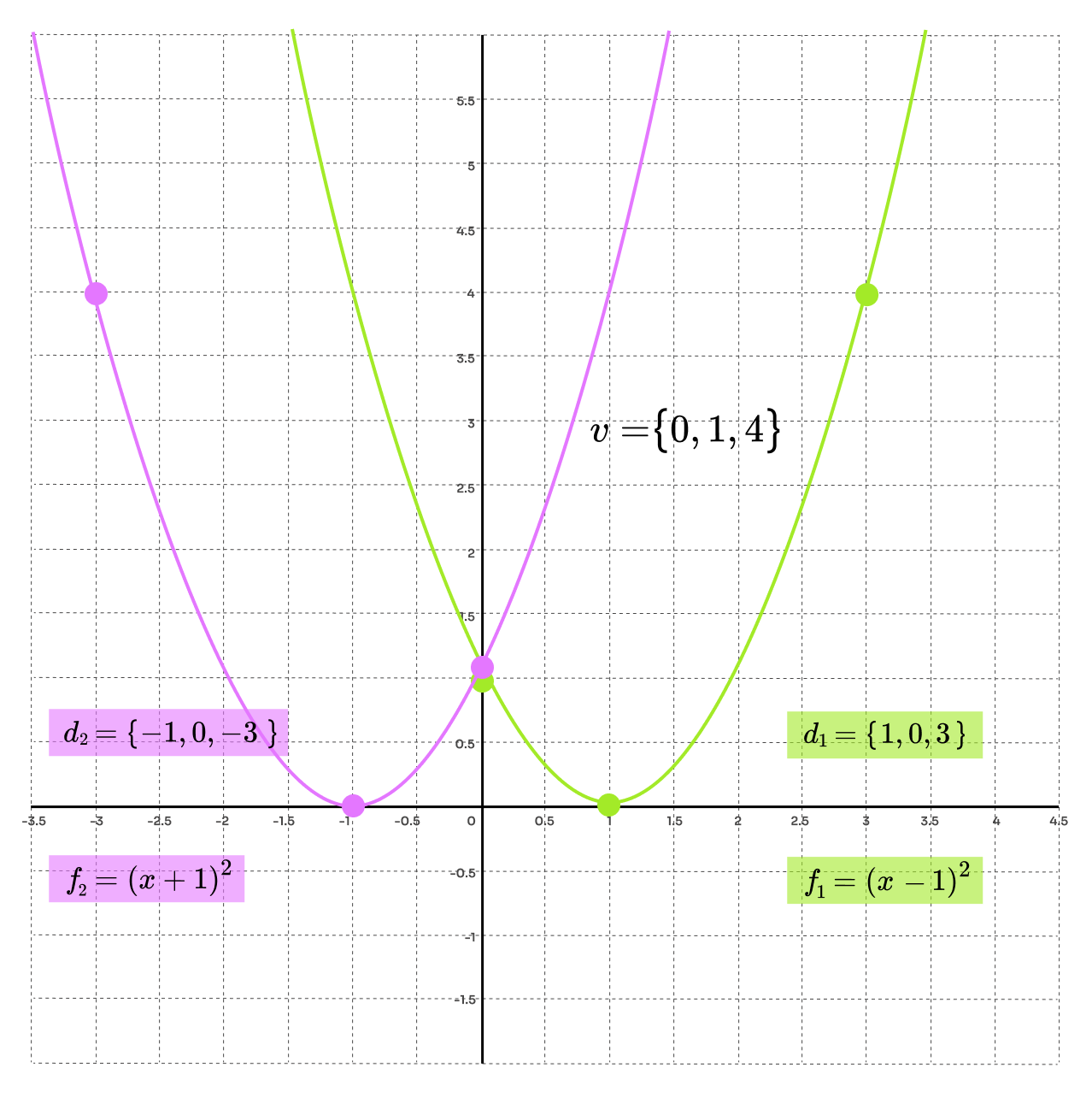
If we pick evaluation domain $d_1$ we get points $(1,0)(0,1)(3,4)$ which define polynomial $(x-1)^2$ while the evaluation domain $d_2$ creates a different set of point $(-1,0)(0,1)(-3,4)$ that define polynomial $(x+1)^2$. By picking an evaluation domain, we get a set of points that uniquely define a polynomial. The domain choice is up to us, and we will use that to our advantage.
All the polynomials we are going to work with are over a finite field $\mathbb{F}_p$. The domain we are going to work with is special because it is generated by primitive $n$-th root of unity $\omega \in \mathbb{F}_p: \omega^n = 1$ as:
$$H = \{\omega^0, \omega^1, \omega^2 ..., \omega^{n-1}\}$$Why should we use this evaluation domain? (optional section)
This domain allows for a more efficient representation of certain polynomials. Let's be more specific. Later in the protocol, we will find great use of the vanishing polynomial $Z_H(x)$, which evaluates to zero over the specified domain $H$. The polynomial has all of the roots from $H$ so it can be written as $Z_H(x) = (x-1)(x-\omega)(x-\omega^2)\ldots(x-\omega^{n-1})$. For large enough $n$, this polynomial gets pretty hard to evaluate. Using $\omega^n = 1$, we can write $Z_H(x) = x^n-1$ in a much nicer representation. But why does it hold? We just need to show that for $\forall x \in H: x^n-1 = 0$:
$$ x = \omega^i : (\omega^i)^n - 1 = (\omega^n)^i - 1 = 1^i - 1 = 0 \text{ thanks to } \omega^n = 1 $$The size of the domain is $n$, which is the number of gates in the circuit, and the size of field $\mathbb{F}_p$ is $p$. In practice, $p$ is much much greater than $n$. The size $p$ is the security parameter, so the bigger it is, the more secure the protocol becomes. Since all of the elements of $H$ are in $\mathbb{F}_p$ and $p \gg n$ it holds that the domain is a subset of the field $H \subset \mathbb{F}_p$.
We already know that any polynomial of degree $d$ could be represented in evaluation form as a set of $d+1$ points. That is pretty neat, but it turns out that we will need to write polynomials in the standard coefficient form $f(x) = c_0 + c_1x + \ldots + c_n c^n$. The problem is that we would like to make KZG commitments where we need to know the coefficient of the polynomial. There are numerous approaches to converting a polynomial from an evaluation form to a coefficient form (interpolating it). We will describe how it can be done using the Lagrange basis because it is easier to explain than the Fourier transform. Given a vector $v$ of size $n$ we can interpolate it over domain $H$ as:
$$v(x) = \sum_{i = 1}^{n} v_i L_i(x)$$where Lagrange basis $L_i(x)$ is a polynomial that is 1 when $x = \omega^i$ and 0 otherwise. For all $\omega^i \in H: v(\omega^i) = v_i$ because in the sum only $L_i(x)$ evaluates to 1 and all other Lagrange bases are 0. This effectively gets us polynomial described by the points:
$$[(1, v_1), (\omega, v_2), (\omega^2, v_3), \ldots, (\omega^{n-1}, v_{n})]$$How does the interpolation work, and what even is $L_i(x)$? (optional section)
Take a polynomial $v(x)$ created from vector $v_i$ by Lagrange interpolation. For input $\omega^i$, only $L_{i}(\omega^i)$ will evaluate to 1, and the remaining Lagrange bases will be zero. Meaning $v(\omega^i) = v_i$, and that is exactly what we want. For the domain $H$, this mysterious basis could be written as:
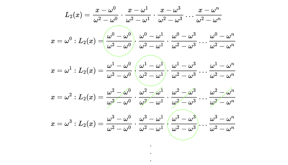
$$L_i(x) = \prod_{k \in H, k \neq \omega^i} \frac{x-k}{\omega^i-k}$$When $x \in H \setminus i$ is plugged into $L_i(x)$, then there is precisely one fraction $\frac{x-k}{\omega^i-k}$ for which $k = x$. In that case, the fraction evaluates to 0, meaning the whole product evaluates to 0. If $x = \omega^i$, the consequence is even more trivial because all of the fractions result in $\frac{\omega^i-k}{\omega^i-k} = 1$, and since $k \neq i$, the product of all fractions results in 1. To convince you it is not complicated, look at the example below with the Lagrange basis $i = 2$.
Lagrange basis can have also sparse representation (with fewer coefficient) on the domain $H$ as described on page 2 of the PlonK paper.
The PlonK paper also describes the protocol with the Lagrange interpolation, but keep in mind that in practice inverse Fast Fourier Transform (iFFT) is used because it is faster. The whole protocol could be even calculated without interpolation as described in Plonk without FFTs.
Common Preprocessed Input
Since the PlonK protocol runs KZG, all of the parties should have access to the information needed in KZG polynomial commitment scheme $(\mathbb{F}_p, \mathbb{G}_1, \mathbb{G}_2, \mathbb{G}_t, e, G_1, G_2, G_t, SRS)$. To revise $\mathbb{F}_p$ is a prime field, $(\mathbb{G}_1, \mathbb{G}_2, \mathbb{G}_t)$ are groups of points on elliptic curves and $e$ is efficiently computable group pairing $e: \mathbb{G}_1 \times \mathbb{G}_2 \rightarrow \mathbb{G}_t$. Lastly $G_1, G_2$ are group generators of $\mathbb{G}_1, \mathbb{G}_2$. Moreover, there needs to be a KZG setup ceremony generating the structured reference string SRS which is public.
Below is summed up the common preprocessed input that is available to both the prover and the verifier. Right now, you do not need to understand how and why it is used, everything will be explained in the following posts.
$n$ number of gates in the arithmetic circuit
$k_1, k_2 \in \mathbb{F}_p$ are needed to create $k_1 H , k_2 H$ such that the union $H' = H \cup k_1 H \cup k_2H)$ contains $3n$ distinct elements. This will be further explained in the round 2.
$SRS$ structured reference string for KZG polynomial commitment scheme
permutation function: $\sigma^*: [3n] \rightarrow H'$ you will see how it is constructed in the round 2
selector polynomials: $q_m(x), q_l(x), q_r(x), q_o(x), q_c(x)$ interpolated from selector vectors $q_m, q_l, q_r, q_o, q_c$ introduced in arithmetization
permutation polynomials: $S_{\sigma_1}, S_{\sigma_2}, S_{\sigma_3}: [n] \rightarrow H'$ interpolated from $\sigma^*$
What do these have in common? They are all dependent just on the structure of the circuit, meaning we could calculate them before the actual execution of the protocol. Now that everything is set up, we can finally start with the first round of the PlonK prover algorithm.